Question 1 (a)
Question 1 (b)
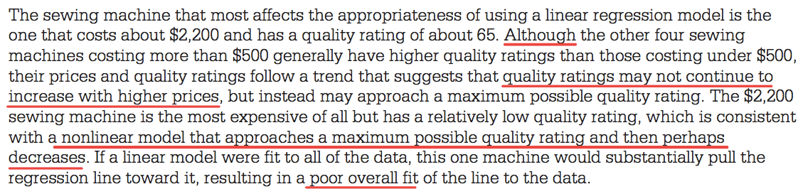
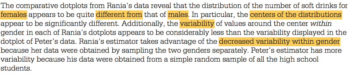
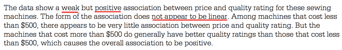
Question 3 (a)
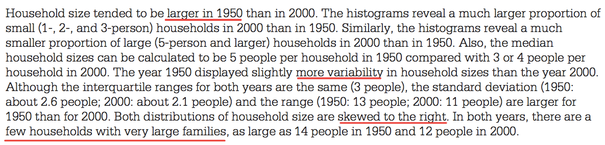
Summarizing Distribution (SOCS)
Shape
- Skewed left/right
Outlier
Q1 - 1.5 * IQR
Q3 + 1.5 * IQR
Center
- Mean or Median
Spread
- SD or IQR
Question 3 (b)
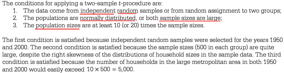
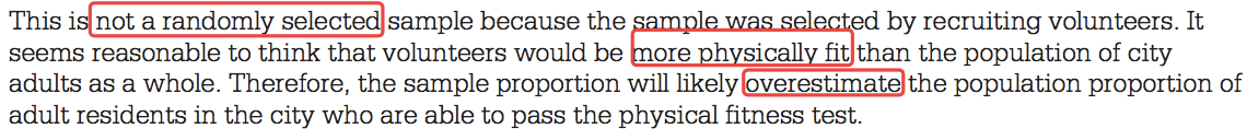
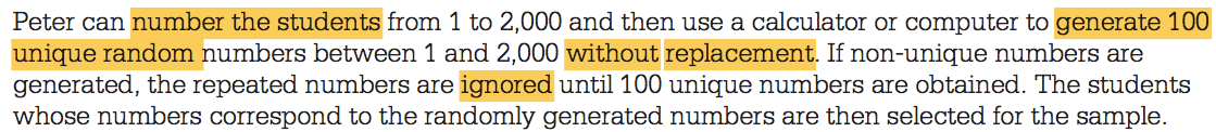
Conditions for Sampling Distribution (RIN)
Random
- How the sample is selected
Independent
N≥10n
N: population size
n: sample size
Normal
For
means
If the population is normally distributed, n can < 30
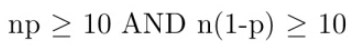
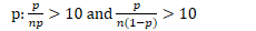
For proportions:
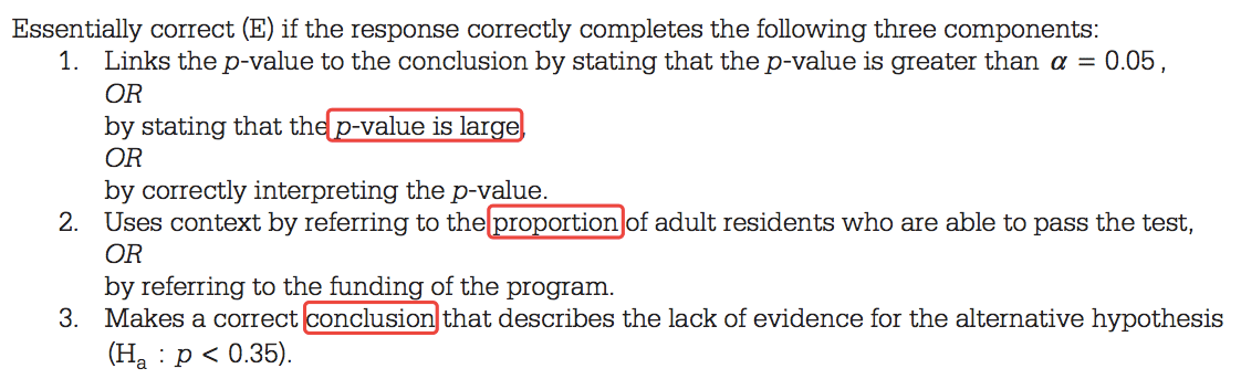
Question 4
Hypothesis Test
Using a Statistic to test a claim about a Parameter
Steps (Why Can't Cat Play Instruments)
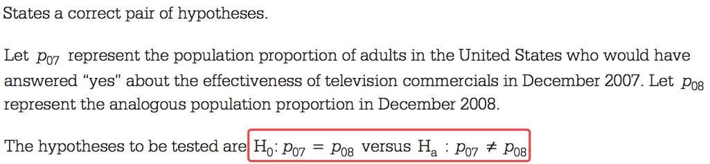
Write the hypothesis
Null hypothesis (H0): Parameter = ____
Alternative hypothesis (H1/Ha): Parameter > or < or ≠ ______
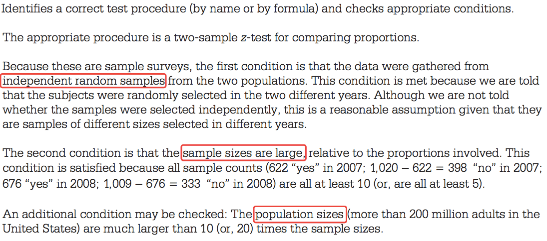
Ckeck conditions (RIN)
Random Sample
Independent: N >10n
Normal:
μ: n≥30
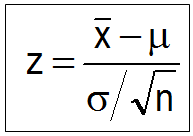
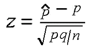
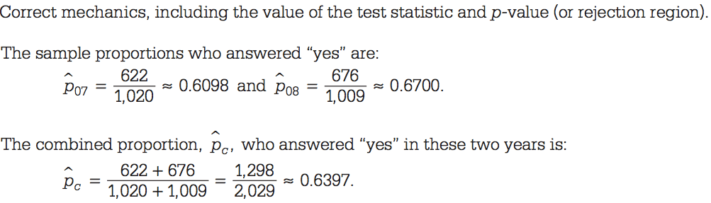
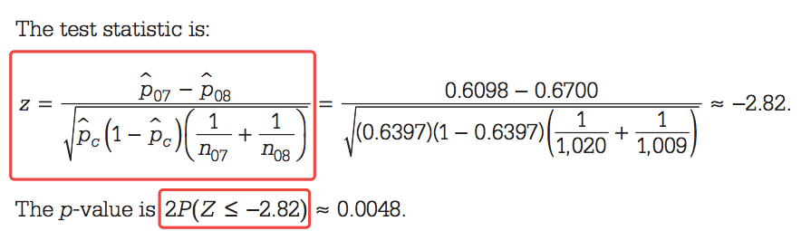
Calculate the test statistic
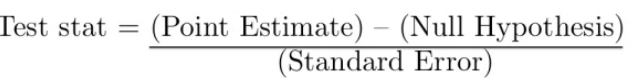
Mean
Proportion
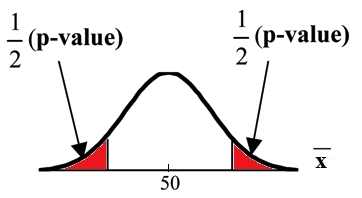
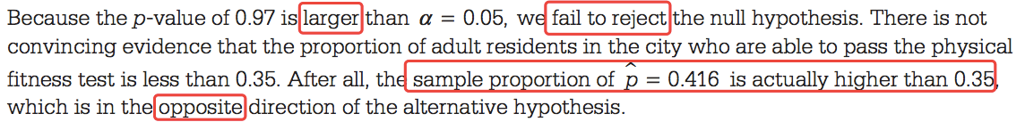
Look up the P-value (from Z table)
- Probability that the null hypothesis (H0) is true, given the sample data you collected
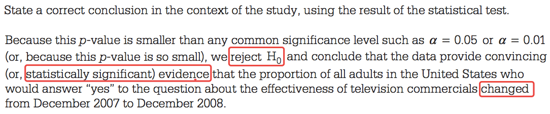
Interpret
| p < α | Reject the null hypothesis | do have evidence to support the claim |
|---|---|---|
| p > α | Fail to reject the null hypothesis | do not have evidence to support the claim |
Step 1
Step 2
Step 3
Step 4
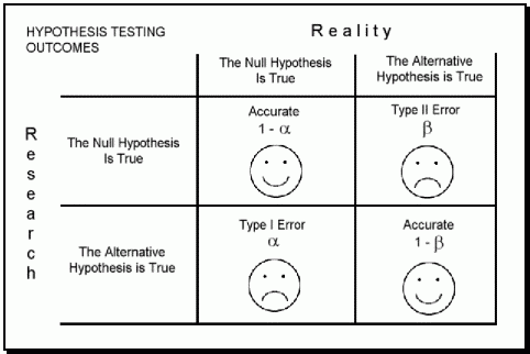
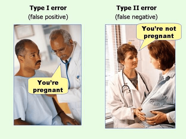
Question 5 (a)
Type I: falsely think alternative hypothesis is true (1 false), DO reject the null hypothesis (1 word)
Type II: falsely think alternative hypothesis is false (2 falses), DO NOT reject the null hypothesis (2 word)
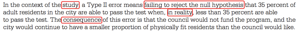
Question 5 (b)
Question 5 (c)
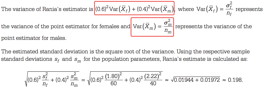
Question 6 (a)
Question 6 (c)
Question 6 (d)